Using Population objects to create biased data

import mlsim
import pandas as pd
import numpy as np
import seaborn as sns
from collections import namedtuple

Create an all default population

pop = mlsim.bias.Population()

To view the details on this population, we can use the get_parameter_description method.

print(pop.get_parameter_description())

Demographic Parameters
DemParams(Pa=[0.5, 0.5], Pz_a=[[0.5, 0.5], [0.5, 0.5]])
Target Parameters 
TargetParams(Py_az=[[[0.95, 0.05], [0.95, 0.05]], [[0.95, 0.05], [0.95, 0.05]]])
Feature Parameters 
FeatureParams(distfunc=<function <lambda> at 0x7f1ffce81040>, theta=[[[[5, 2], [2, 5]], [[5, 2], [2, 5]]], [[[5, 2], [2, 5]], [[5, 2], [2, 5]]]])
Feature Noise Parameters 
NoiseParams(noisefunc=<function <lambda> at 0x7f1ffce81dc0>, theta=[[[1.0, 1.0], [1.0, 1.0]], [[1.0, 1.0], [1.0, 1.0]]])

The instantiation just assigns values to these parameters. In order to get data, we use the sample method.

help(pop.sample)

Help on method sample in module mlsim.bias.populations:

sample(N, return_as='DataFrame') method of mlsim.bias.populations.Population instance
    sample N members of the  population, according to its underlying
    distribution
    
    Parameters
    -----------
    N : int
        number of samples
    return_as : string, 'dataframe'
        type to return as, can be pandas 'DataFrame' or IBM AIF360
        'structuredDataset'

pop_df1 = pop.sample(100)
pop_df1.head()

	a	z	y	x0	x1
0	0.0	0.0	1.0	4.251619	3.227683
1	0.0	1.0	1.0	0.623027	5.995485
2	0.0	1.0	1.0	2.597801	4.980416
3	1.0	1.0	1.0	0.132915	6.271830
4	1.0	1.0	1.0	4.358112	2.214810

Changing the type of bias

Now demo some with various biases to create examples

# create a correlated demographic sampler
label_bias_dem = mlsim.bias.DemographicCorrelated(rho_a=.2,rho_z=[.25,.15])

# instantiate a population with that
pop_label_bias = mlsim.bias.PopulationInstantiated(demographic_sampler=label_bias_dem)

pop_label_bias_df1 = pop_label_bias.sample(100)
pop_label_bias_df1.head()

	a	z	y	x0	x1
0	1.0	0.0	0.0	4.024818	1.580869
1	0.0	0.0	0.0	6.641384	1.888501
2	1.0	0.0	0.0	4.628367	-0.202582
3	0.0	0.0	0.0	4.884726	0.487902
4	0.0	0.0	0.0	5.910277	-0.245840

New we’ll create a feature bias where the classes are separable for one group and not for the other.

feature_sample_dist = lambda mu,cov :np.random.multivariate_normal(mu,cov)
per_group_means = [[[1,2,3,4,3,3],[4,6,8,8,10,6]],[[3,2,3,4,4,3],[1,3,4,4,5,3]]]
D =6
shared_cov = [np.eye(D)*.75,.95*np.eye(D)]
feature_bias = mlsim.bias.FeaturePerGroupSharedParamWithinGroup(
            feature_sample_dist,per_group_means,shared_cov)
pop_feature_bias = mlsim.bias.PopulationInstantiated(feature_sampler=feature_bias)

pop_feature_bias_df1 = pop_feature_bias.sample(100)
pop_feature_bias_df1.head()

	a	z	y	x0	x1	x2	x3	x4	x5
0	0.0	1.0	1.0	4.711952	6.212549	10.054750	7.584091	8.150176	6.558052
1	1.0	1.0	1.0	0.660586	1.098325	6.264511	5.848877	3.606027	3.143128
2	0.0	1.0	1.0	1.802936	4.084537	8.315621	5.176766	10.405194	9.535016
3	0.0	0.0	0.0	0.630422	1.976371	4.002007	3.166266	0.437942	3.548206
4	1.0	0.0	0.0	4.393422	1.548517	1.455341	6.558026	5.040535	1.810092

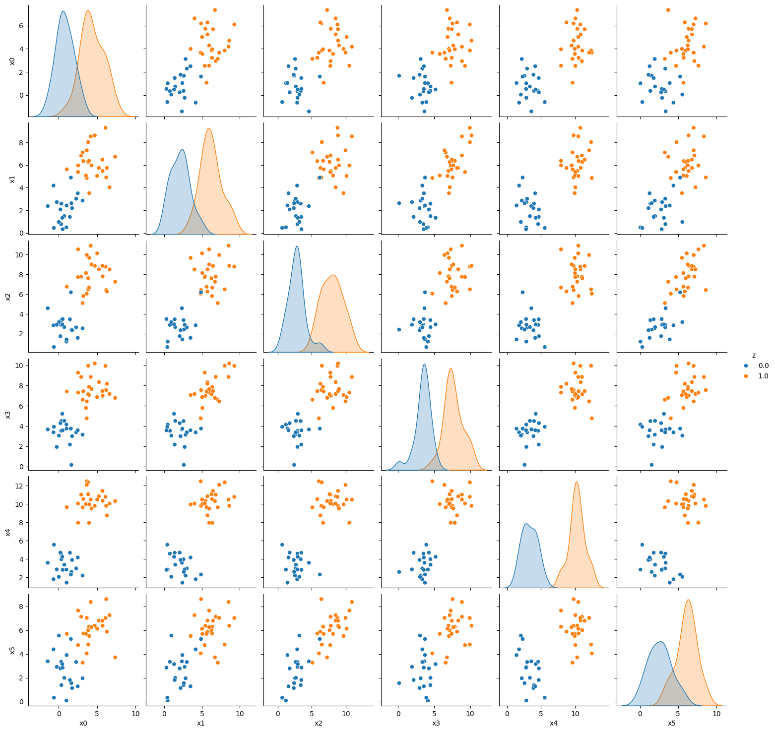
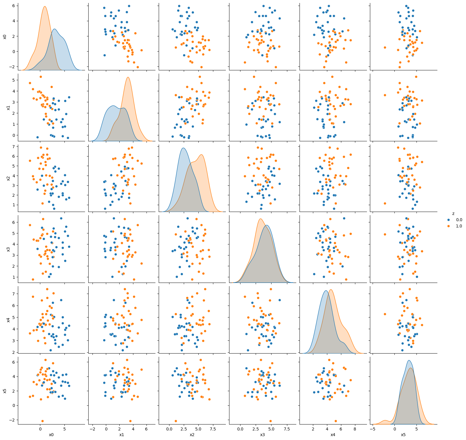
var_list = ['x'+ str(i) for i in range(D)]
g = sns.pairplot(pop_feature_bias_df1, vars= var_list, hue = 'z')

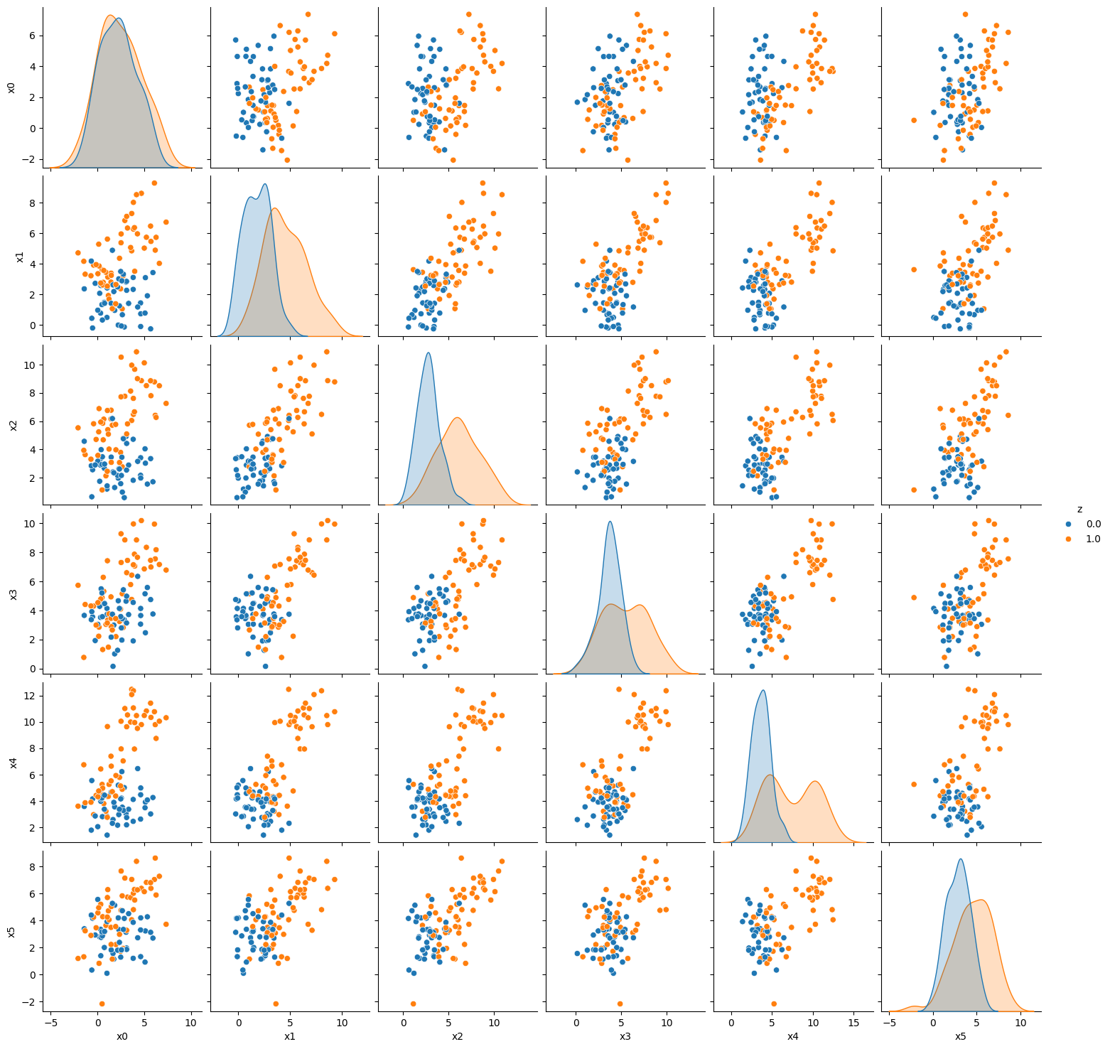
[sns.pairplot(dffbai, vars= var_list, hue = 'z') for ai,dffbai in pop_feature_bias_df1.groupby('a')]

[<seaborn.axisgrid.PairGrid at 0x7f1ff5654e80>,
 <seaborn.axisgrid.PairGrid at 0x7f1ff5e1f2b0>]